Can we train high-quality models on distributed, privacy-sensitive data without compromising security? Federated learning aims to solve this problem by training models locally and aggregating updates, but there’s a catch—shared model parameters or probabilistic predictions (soft labels) still leak private information. Our new work, “Little is Enough: Boosting Privacy by Sharing Only Hard Labels in Federated Semi-Supervised Learning,” presents an alternative: federated co-training (FedCT), where clients share only hard labels on a public dataset.
This simple change significantly enhances privacy while maintaining competitive performance. Even better, it enables the use of interpretable models like decision trees, boosting the practicality of federated learning in domains such as healthcare.
Federated learning (FL) is often praised for enabling collaborative model training without centralizing sensitive data. However, model parameters can still leak information through various attacks, such as membership inference and gradient inversion. Even differentially private FL, which adds noise to mitigate these risks, suffers from a trade-off—stronger privacy means weaker model quality.
Another alternative, distributed distillation, reduces communication costs by sharing soft labels on a public dataset. While this improves privacy compared to sharing model weights, soft labels still expose patterns that can be exploited to infer private data.
This brings us to an essential question: Is there a way to improve privacy without sacrificing model performance?
A Minimalist Solution: Federated Co-Training (FedCT)
Instead of sharing soft labels, FedCT takes a radical yet intuitive approach: clients only share hard labels—definitive class assignments—on a shared, public dataset. The server collects these labels, forms a consensus (e.g., majority vote), and distributes the pseudo-labels back to clients for training.
This approach has three key advantages:
Stronger Privacy – Hard labels leak significantly less information than model parameters or soft labels, drastically reducing the risk of data reconstruction attacks.
Supports Diverse Model Types – Unlike standard FL, which relies on neural networks for parameter aggregation, FedCT works with models like decision trees, rule ensembles, and gradient-boosted decision trees.
Scalability – Since only labels are communicated, the approach dramatically reduces bandwidth usage—by up to two orders of magnitude compared to FedAvg!
Empirical Results: Privacy Without Performance Trade-Offs
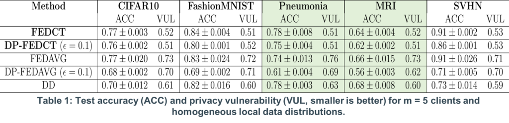
We evaluated FedCT on various benchmark datasets, including CIFAR-10, Fashion-MNIST, and real-world medical datasets like MRI-based brain tumor detection and pneumonia classification.
Key Findings:
Privacy wins: FedCT achieves near-optimal privacy (VUL ≈ 0.5), making membership inference attacks no better than random guessing.
Competitive accuracy: FedCT performs as well as, or better than, standard FL and distributed distillation in most scenarios.
Interpretable models: It successfully trains decision trees, random forests, and rule ensembles, unlike other FL approaches.
Robust to data heterogeneity: Even when clients have diverse (non-iid) data, FedCT performs comparably to FedAvg.
Notably, FedCT also shines in fine-tuning large language models (LLMs), where its pseudo-labeling mechanism outperforms standard federated learning.
Privacy Through Simplicity
The core idea behind FedCT is beautifully simple: share less, retain more privacy. By moving away from parameter sharing and probabilistic labels, we mitigate privacy risks while keeping performance intact.
That said, some open questions remain:
How does the choice of public dataset impact FedCT’s effectiveness?
Can we further refine the consensus mechanism for extreme data heterogeneity?
How does FedCT behave when applied to real-world hospital collaborations?
For now, our results suggest that in federated learning, little is enough. Sharing only hard labels provides a surprisingly strong privacy-utility trade-off—especially in critical applications like healthcare.
Linear mode connectivity describes a phenomenon observed for neural networks where every linear interpolation between two trained neural networks has roughly the same loss. In other words, there is a rather flat line in the loss surface connecting the two networks.
We know that linear mode connectivity (LMC) doesn’t hold for two independently trained models. But what about layer-wise LMC? Well, it is very different! Our new work “Layer-wise linear mode connectivity” published at ICLR 2024 explores this and its applications to federated averaging. This is joint work led by Linara Adylova, together with Maksym Andriushchenko, Asja Fischer, and Martin Jaggi.
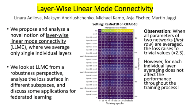
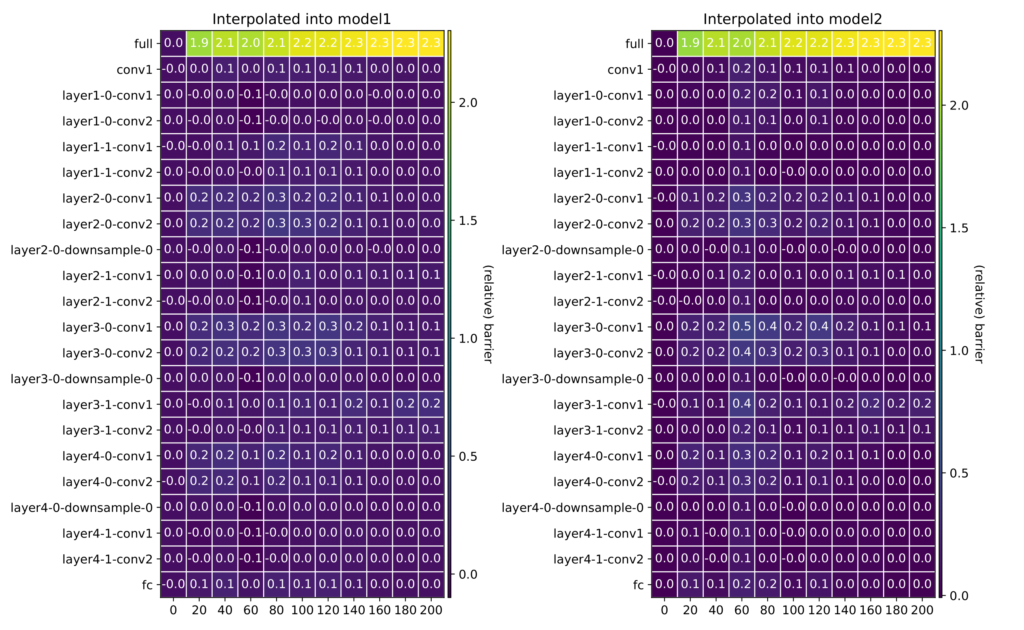
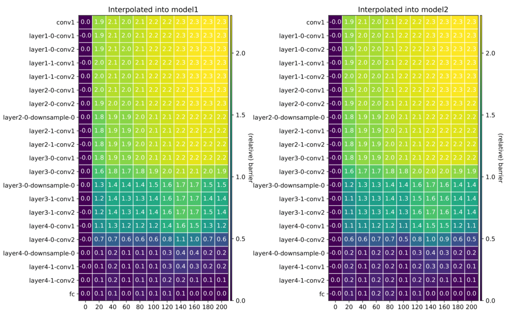
We investigate layer-wise averaging and discover that for multiple networks, tasks, and setups averaging only one layer does not affect the performance (See Fig. 2). This is in line with the research of Chatterji, at al. [1] showing that reinitialization of individual layers does not change accuracy.
Figure 2: Layer-wise barriers between two models.
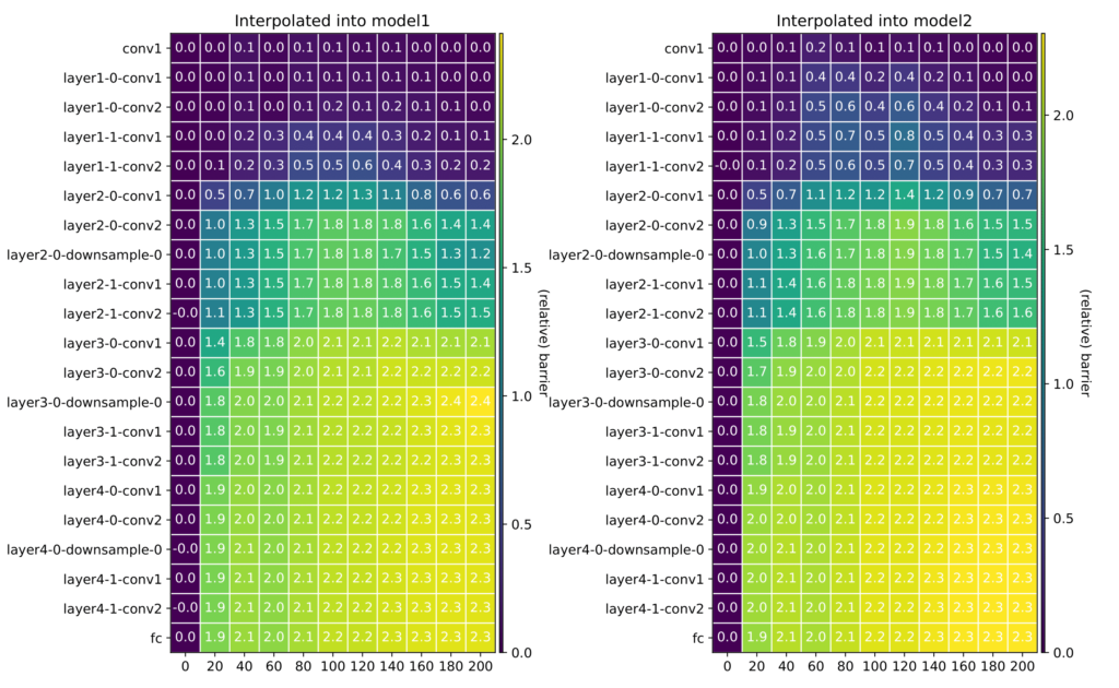
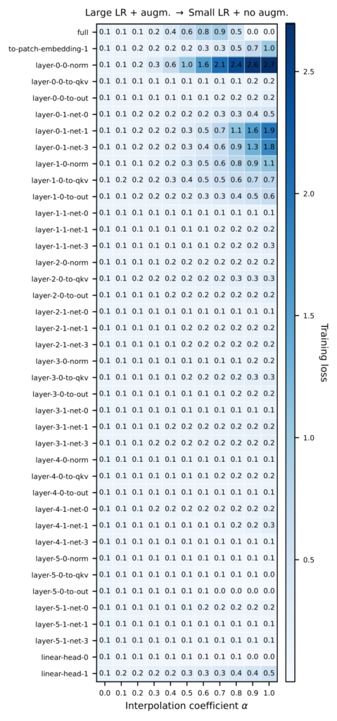
Nevertheless, one might as whether there is some critical amount of layers needed to be averaged to get to a high loss point. We investigated this in Fig. 3 by computing the barrier when interpolating between the first layers of the two networks, then the first and second layer, and so on (left). We did the same starting from the bottom, interpolating between the last layers, then the last and penultimate layers, and so on (right). It turns out that barrier-prone layers are concentrated in the middle of a model.
Figure 3: Cumulative Barriers.
(left: from the top, right: from the bottom)
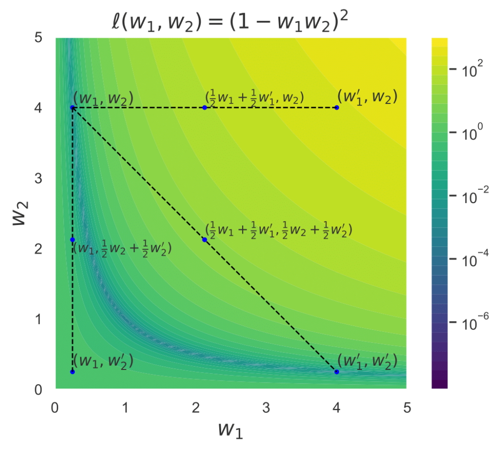
Is there a way to gain more insights on this phenomenon? Let’s see how it looks like for a minimalistic example of a deep linear network (Fig. 4). Ultimately, a linear network is convex with respect to any of its layer cuts. This example demonstrates how the interpolation between the full networks leads to a barrier, while interpolating only the second layer leads to a much lower loss barrier. Interpolating only the first layer, however, leads to a high loss barrier, consistent with our experiments on deep non-linear networks.
Figure 4: Example of LLMC with a 1D diagonal linear network.
Figure 5: Robustness to random perturbations.
Can robustness explain this property? That is, do all the neural networks have a particular weight changes robustness that allows to compensate for one layer modifications? Or is the interpolation direction somehow special? We tested the robustness to random perturbations of each layer in Fig. 5. Our results show that for some layers there is indeed a robustness against perturbations. Moreover, the more robust the model is in general, e.g., because being in a flat minimum [2], the harder it is to get a high loss through perturbations. However, we do not see the same behavior of layers for random perturbation that we see for the interpolation between two networks. This indicates that the interpolation direction is indeed somehow special.
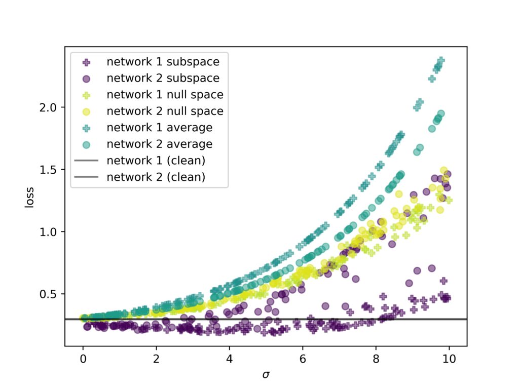
This means, we cannot treat random directions as uniformly representative of the loss surface. To investigate this further, we analyze how loss in different directions impacts the loss of a network. We distinguish three separate directions: (i) a random perturbation along the interpolation direction, (ii) in the training subspace, i.e., the space spanned by the two networks during training, and (iii) the null space, i.e., the subspace perpendicular to the training subspace. Our experiment in Fig, 6 shows that particular subspaces are more stable than others. Especially, the interpolation direction is susceptible to noise.
Figure 6: Impact of random perturbation in different subspaces on the loss of a neural network.
In summary, we investigate the fine-grained structure of barriers on the loss surface observed when averaging models. We propose a novel notion of layer-wise linear mode connectivity and show empirically that on the level of individual layers the averaging barrier is always insignificant compared to the full model barrier. We also discover a structure in the cumulative averaging barriers, where middle layers are prone to create a barrier, which might have further connections to the existing investigations of the training process of neural networks.
It is important to emphasize that the definition of barrier should be selected very carefully: When performance of the end points is very different, comparing to the mean performance might be misleading for understanding the existence of barrier. Our explanation of LLMC from the robustness perspective aligns with previously discovered layer criticality [3] and shows that indeed more robust models are slower to reach barriers. Training space analysis indicates that considering random directions on the loss surface might be misleading for its understanding.
Our research poses an interesting question: How is the structure of barriers affected by the optimization parameters and the training dataset? We see a very pronounced effect of learning rate and in preliminary investigation we observe that easier tasks result in less layers sensitive to modifications. Understanding this connection can explain the effects of the optimization parameters on the optimization landscape.
References: [1] Niladri S Chatterji, Behnam Neyshabur, and Hanie Sedghi. The intriguing role of module criticality in the generalization of deep networks. In International Conference on Learning Representations, 2020. [2] Henning Petzka, Michael Kamp, Linara Adilova, Cristian Sminchisescu, and Mario Boley. Relative flatness and generalization. In Advances in Neural Information Processing Systems, 2021. [3] Zhang, Chiyuan, Samy Bengio, and Yoram Singer. “Are all layers created equal?.” The Journal of Machine Learning Research 23.1 (2022): 2930-2957.
How can we learn high quality models when data is inherently distributed across sites and cannot be shared or pooled? In federated learning, the solution is to iteratively train models locally at each site and share these models with the server to be aggregated to a global model. As only models are shared, data usually remains undisclosed. This process, however, requires sufficient data to be available at each site in order for the locally trained models to achieve a minimum quality – even a single bad model can render aggregation arbitrarily bad.
In healthcare settings, however, we often have as little as a few dozens of samples per hospital. How can we still collaboratively train a model from a federation of hospitals, without infringing on patient privacy?
At this year’s ICLR, my colleagues Jonas Fischer, Jilles Vreeken and me presented an novel building block for federated learning called daisy-chaining. This approach trains models consecutively on local datasets, much like a daisy chain. Daisy-chaining alone, however, violates privacy, since a client can infer from a model upon the data of the client it received it from. Moreover, performing daisy-chaining naively would lead to overfitting which can cause learning to diverge. In our paper “Federated Learning from Small Datasets“, we propose to combine daisy-chaining of local datasets with aggregation of models, both orchestrated by the server, and term this method Federated Daisy-Chaining (FedDC).
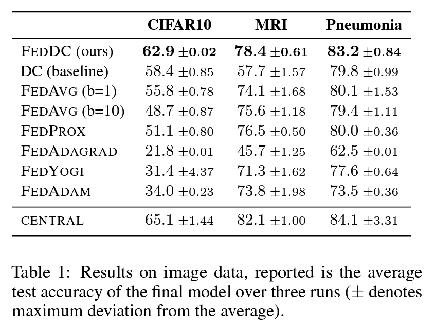
This approach allows us to train models successfully from as little as 2 samples per client. Our results on image data (Table 1) show that FedDC not only outperforms standard federated avering (FedAvg), but also state-of-the-art federated learning approaches, achieving a test accuracy close to centralized training.
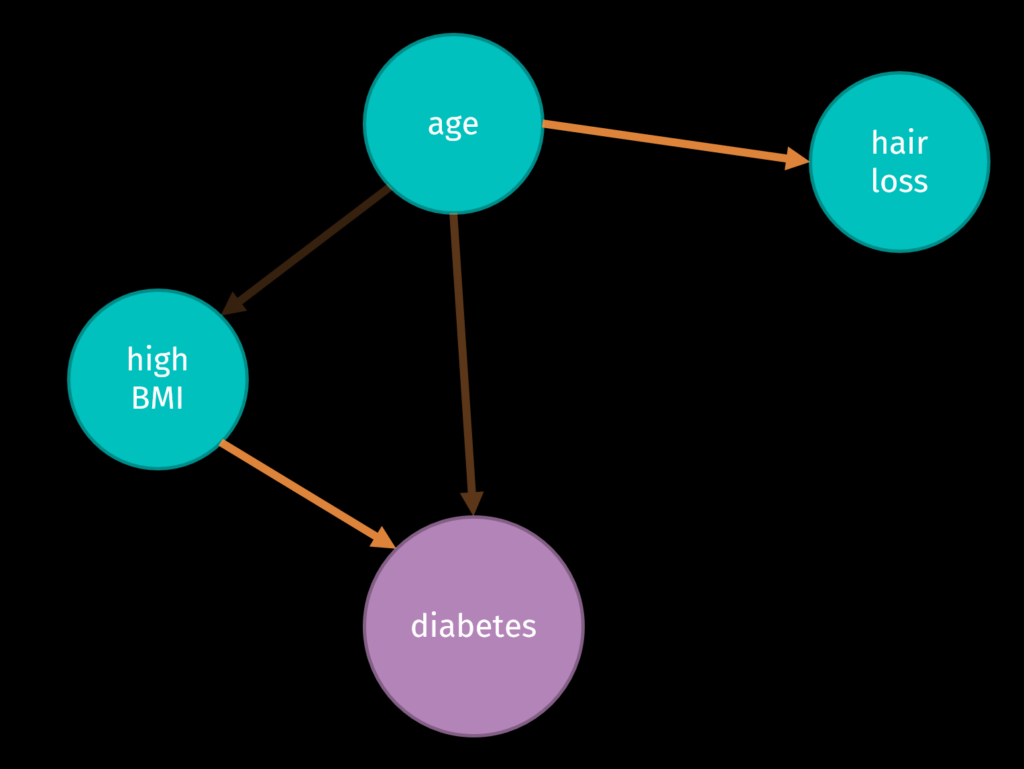
Discovering causal relationships enables us to build more reliable, robust, and ultimately trustworthy models. It requires large amounts of observational data, though. In healthcare, for most diseases the amount of available data is large, but this data is scattered over thousands of hospitals worldwide. Since this data in most cases mustn’t be pooled for privacy reasons, we need a way to learn a structural causal model in a federated fashion.
At this year’s AISTATS, my co-authors Osman Mian, David Kaltenpoth, Jilles Vreeken and me presented the paper “Nothing but Regrets – Privacy-Preserving Federated Causal Discovery” in which we show that you can discover causal relationships by sharing only regret values with a server: The server sends a candidate causal model to each client and the clients reply with how much worse single-edge extensions of this global model are compared to the original global model. From this information alone, the server can compute the best extension of the current global model.
In practice, the environments at the local clients are not the same. We should expect local differences that could be modeled by interventions into the global causal structure. In our AAAI paper “Information-Theoretic Causal Discovery and Intervention Detection over Multiple Environments” we have shown how to discover a global causal structure as well as local interventions in a centralized setting. Our current goal is to combine these two works to provide an approach to federated causal discovery from heterogeneous environments.
At AAAI 2023 my colleagues Osman Mian, Jilles Vreeken and me presented our paper “Information-Theoretic Causal Discovery and Intervention Detection over Multiple Environments” in which we learn a global structural causal model over multiple environments, as well as discover potential local intervention that change some causal relationships within particular environments.
For medical data this has an enormous impact: Being able to reliably detect causal relationships in medical data, such as gene expressions or patient records, allows us not only to build more reliable and trustworthy models, but also to detect novel insights on diseases and risk factors.
Reliably detecting causal relationships requires large amounts of observational data, though. Therefore, it is paramount to develop privacy-preserving methods to tap into the large, but inherently distributed medical datasets in hospitals all over the world. What we need is federated causal discovery.
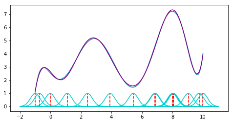
To explain the kernel trick to students at Monash University, I once created a jupyter notebook that explains the basics with a few illustrations. I embed the notebook below, but you can also view it directly, or check it out on github. It is all part of my Machine Learning Explained repository, where I collect little bits of information on machine learning.
Disclaimer: this article is an advertisement for our workshop on parallel, distributed, and federated learning (PDFL’20) at ECMLPKDD this year and a call for contributions. First I wanted to just post the workshop description and be done with it, but then I thought I might add some actual content to give this article some actual value. Let’s see how that works out.
Distributed Machine Learning
Distributed machine learning is a huge topic since the Big Data hype. However, the landscape of machine learning applications is changing rapidly: large centralized datasets are replaced by high volume, high velocity data streams generated by a vast number of geographically distributed, loosely connected devices, such as mobile phones, smart sensors, autonomous vehicles or industrial machines. Current learning approaches centralize the data and process it in parallel in a cluster or cloud. This way, you again have a centralized dataset and can run your off-the-shelf efficient machine learning algorithm – think of Spark’s mllib, for example. And of course, a lot of really good research is done on how to improve machine learning in such a high-performance setup (e.g., the work of Janis Keuper). However, this has three major disadvantages: (i) it does not scale well with the number of data-generating devices since their growth exceeds that of computing centers, (ii) the communication costs for centralizing the data are prohibitive in many applications, and (iii) it requires sharing potentially privacy-sensitive data. Pushing computation towards the data-generating devices alleviates these problems and allows to employ their otherwise unused computing power.
Distributed Gradient Computation
The first more general parallelization scheme, i.e., one that is applicable to several ML algorithms at once, was the distributed mini-batch algorithm of Ofer Dekel and his colleagues from Microsoft (I think the idea precedes him, but he wrote the seminal paper). The idea is very simple: in any gradient based ML algorithm, e.g., stochastic gradient descent, you can calculate the gradients locally and send them to a coordinator node. The coordinator sums them up (which is theoretically sound, since the sum of local gradients is the gradient with respect to all local data points) and performs one update step with the summed up gradient. It then sends the updated model to the local nodes who compute the next round of gradients. There’s been extensive work on showing why this is theoretically sound, and it actually works in practice. The scalability of the approach is seemingly perfect, and it has even been called “embarrassingly parallel”, to underline how easy and effective the parallelization is. Since a lot of machine learning relies on gradient based methods, this technique is wide-spread, e.g., it is used in Spark’s mllib and in many implementations of the parameter server.
The Problem of Distributed Gradient Computation for ML
At this point, we could be done. Actually, during my PhD I at many points asked myself why I should work on other methods, since this is so effective. But the devil lies in the detail, and there are two large, connected issues with this technique. The first one is the amount of communication: for every update step, the locally computed gradients need to be send to the coordinator and the updated model has to be send back. This is no problem in a tightly connected system, like a high-performance cluster, but can already become an issue in a cloud, and is prohibitive for physically distributed devices, like cars and cellphones. So why not compute more local gradients each iteration and update a bit less frequently? On paper, this should solve the problem. Here comes the second, more severe issue into play. And for this one, I have to give a bit of background.
Two very prominent optimization algorithms used for machine learning are gradient descent (GD) and stochastic gradient descent (SGD). In gradient descent, you compute the gradient with respect to all samples in your dataset and then update your model, and keep iterating this until you converge. In stochastic gradient descent, you compute the gradient with respect to only a single sample and then update. In standard optimization settings, GD requires less updates, but each update is more costly, since you have to calculate all the gradients. SGD instead requires more updates, but each update is dirt cheap. There is also something in between, the mini-batch SGD: compute the gradient with respect to a hand full of samples (the mini-batch) and then update. The larger the mini-batch, the more this resembles GD, the smaller it is, the more it behaves like SGD.
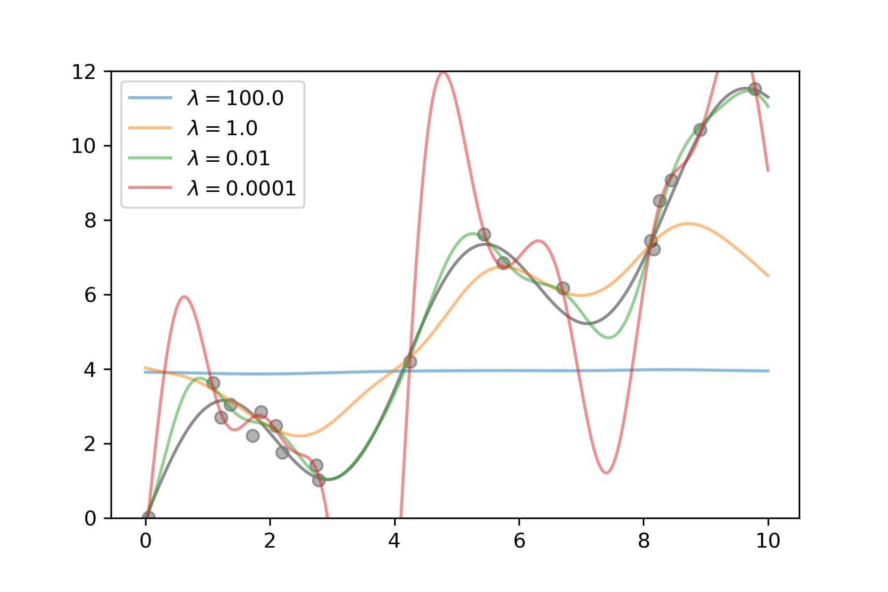
Figure 1: Support vector regression of a one-dimensional example (sinus with upward trend) trained on a sample of 20 points. The higher the regularization parameter lambda, the less complex the model gets, up to a horizontal line for lambda = 100. The smaller the parameter, the more complex the model becomes, eventually being able to fit nearly each sample point, but behaving wildly wrong in-between samples.
With machine learning, there is however an interesting twist to the story, and this one becomes more theoretical, so please bear with me. In machine learning, you want to optimize the risk, or true error of your model. That is, you want to minimize the error the model makes on novel, unseen data. This is also called the generalization error. All that you can do, however, is minimize the empirical error, that is, the error you make on your training set. However, simply finding the model that minimizes the empirical risk can lead to an effect called overfitting: if the model is complex enough, it can memorize the training set and achieve zero error there, but be completely wrong on everything else. What is typically done to avoid this is called regularization: you restrict the model complexity a bit to find a nice trade-off between empirical error and generalization. In figure 1 I illustrate this for support vector machines. Their complexity can be controlled with the regularization parameter lambda. If we regularize too much, the model is very simple and cannot fit the data, so both empirical and true error are high. If we regularize too little, the model becomes very complex and can fit each training point nearly perfectly, but in between it shows crazy behavior. The optimum is somewhere in the middle. Of course, finding this optimum is not trivial and has to be done empirically for each new dataset.
Ok, so why this lengthy digression into generalization? Because SGD has a very cool property: if you draw a new sample for every update, then in expectation, SGD optimizes the true error directly, not the empirical error (see Chapter 14.5.1 in this awesome book). So while GD is better at finding the model that minimizes the empirical error, SGD will find a model that does not minimize the empirical error, but generalizes a lot better. And indeed, this has been observed over and over, especially with neural networks. And now, finally, we get back to the problem with distributed mini-batching. When you calculate more gradients on each local device, the update is made with respect to more samples. So your “mini-batch size” becomes larger. But then, your learning algorithm behaves more like GD and not like SGD. So your model’s true error will become worse. And it’s not only the communication frequency, it’s also the number of nodes. If you have 10 nodes, and each one computes a single gradient, then the effective mini-batch size for your updates is 10. If you use 1000 nodes each computing a single gradient, the mini-batch size becomes 1000. So here is the gist: with distributed mini-batching you cannot scale up your system arbitrarily and you cannot reduce communication that much, because otherwise it will behave too much like GD and will produce models that do not generalize well. Short disclaimer at this point: I am sure that lots of people have worked on clever practical tweaks to alleviate this problem and I hope we will see some of these at our workshop. However, there is no principle way around it – at least I don’t know of one, so please correct me if I am wrong.
Model Averaging and Federated Learning
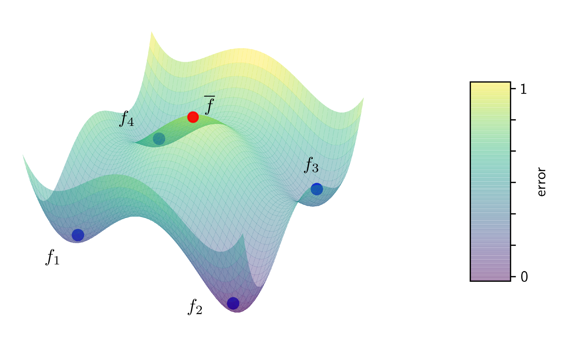
Figure 2: Illustration of a non-convex error surface with four models (blue) each having reached a local minimum. The average (red) of these models has a substantially higher error than any of the four local models.
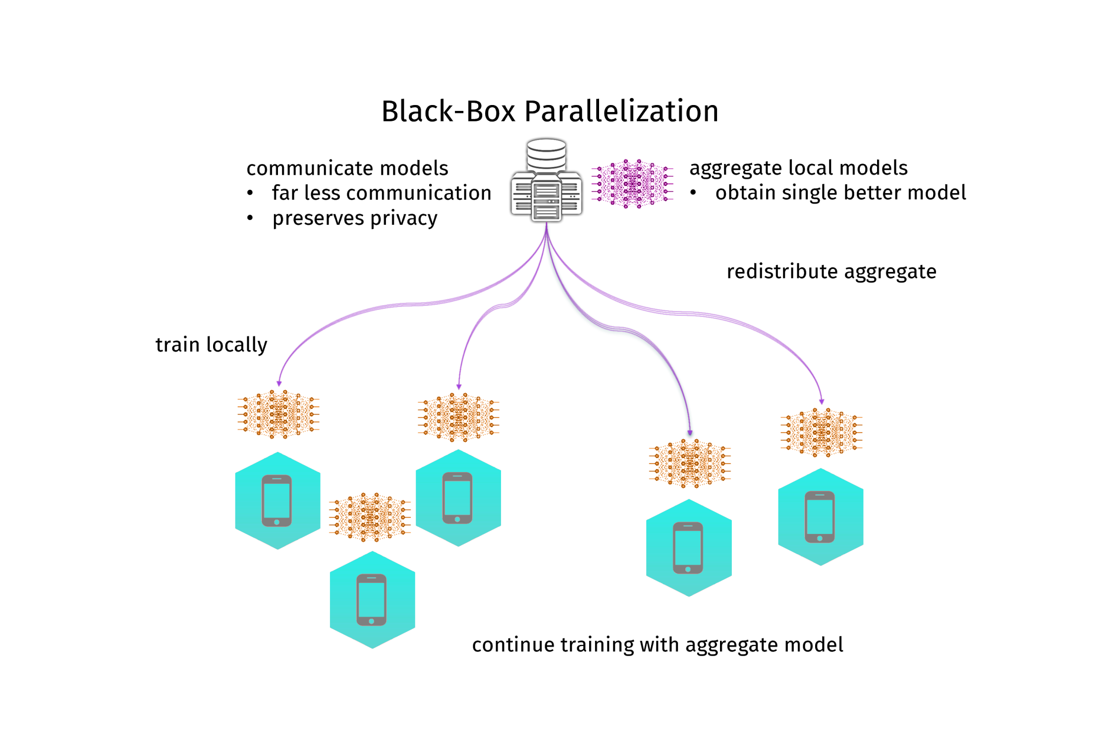
A different approach is to not parallelize the learning algorithm itself at all. Instead, you train a local model, send the model parameters to the coordinator and aggregate them into a better model (and then you could send that better model back and iterate the process). In my PhD-thesis I called this black-box parallelization, since it treats the learning algorithm as a black box. A simple but effective method to aggregate model parameters is to just average them. A lot of people where researching in this direction, but it was Google that brought the breakthrough in 2017 and gave this approach popularity, when they did averaging for neural networks and called it federated learning. This has created quite a hype around this topic, especially in the deep learning community. And indeed, it works. Google is using it to train their link recommendation models in their keyboard app for android phones. It uses less communication and is more resilient than distributed mini-batching. Moreover, this approach is highly privacy-preserving, and thus a hot candidate for machine learning in the medical domain. However, there is one big issue: the model you get by averaging is not necessarily the one you would get from centralized training. Instead, you always loose in model quality. And this time not only on the generalization ability, but actually also on the empirical error. It gets even worse: for neural networks there can be multiple minima of the empirical error, so the average of a bunch of models can be even a lot worse than the local models (see figure 2 for an illustration). In practice, this still works very well. Moreover, the communication can be further reduced by only communicating with a random subset of nodes (federated averaging), or by deciding in a data-driven manner when to communicate (dynamic averaging). And under some strict assumptions, one can even understand how it works theoretically.
Still, there is one subtle issue which might be a deal breaker. Let’s assume we learn using our off-the-shelf SGD which requires us to set a learning rate, let’s call that one l. It is the step size each update makes. To achieve good performance, this l has to be set correctly, not too small and not to large. If we choose it too small, the algorithm will take ages to converge to a good model. If we choose it too large, the algorithm will jump around wildly and might ultimately diverge, breaking the learning entirely. Now, what happens when you train two models separately, each with a learning rate l for exactly one update step and then average their parameters? You will get the same model you would get when training on both local datasets jointly, but with half the learning rate. If instead you used ten models, it would be one tenth the learning rate (see Prop. 3 in this paper on dynamic averaging for deep learning). So the learning rate goes down with the number of nodes in your distributed system. Now this is a huge problem! If you use too many nodes, your effective learning rate will be tiny and the model barely converges to a good one. One can compensate by setting higher learning rates at the local nodes – and this actually works – but it only goes so far; if you set the local learning rates too high, local training breaks completely and nothing works. This seems to put a limit on the scalability of the approach. I would love to see some analysis and ideas to overcome this in our workshop!
The Radon Machine
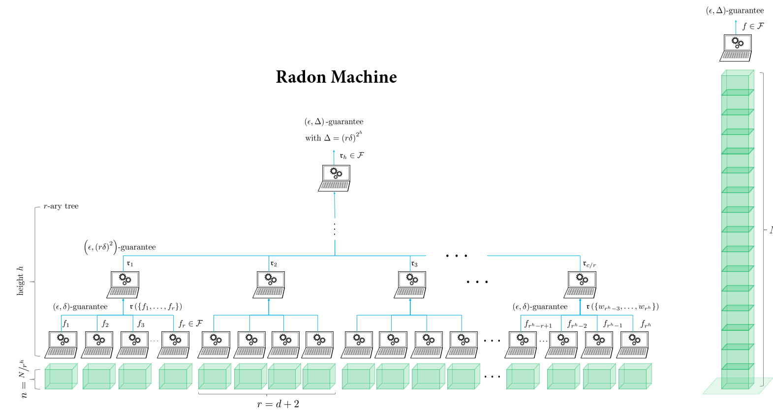
Finally, there is a more esoteric approach which does not average model parameters but iteratively calculates a form of high-dimensional median – called the Radon point – on them. The approach is called Radon machine and has some very nice theoretical properties. It scales well with the number of nodes, it gives a guarantee on the model quality, it is also privacy preserving, and it only requires a single round of communication. However, it currently only works for linear models and the guarantees only hold for convex learning problems. So its practical use is still quite limited. Still, going beyond averaging could be the way to overcome all these issues. I hope we can see some novel approaches along this line, as well.
Conclusion
So here we are: there are traditional distributed ML approaches that produce the same model as the centralized computation, but they require a prohibitive amount of communication and don’t scale well. Then there is distributed mini-batching, which computes gradients in parallel. This is working well in tightly coupled systems like high-performance clusters, but works not so well on physically distributed devices and doesn’t arbitrarily scale. Then there is model averaging, which works well in practice, but is not well understood theoretically, and seems to have an in-built limit to its scalability. And then there is the Radon machine, which is theoretically interesting, but limited to convex methods and linear models, so at its current stage it is not very useful in practice. Thus, despite the surge of papers in this phase of hype, there is still a lot to do. And with this, I will now blatantly advertise our workshop.
Workshop on Parallel, Distributed, and Federated Learning – PDFL’20